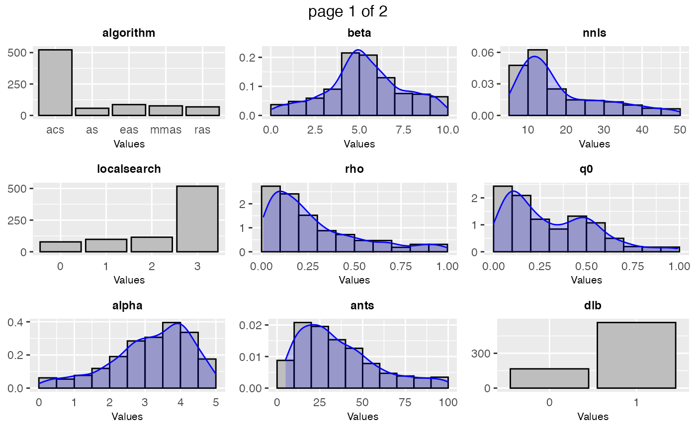
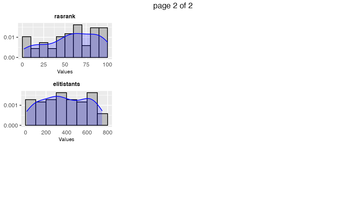
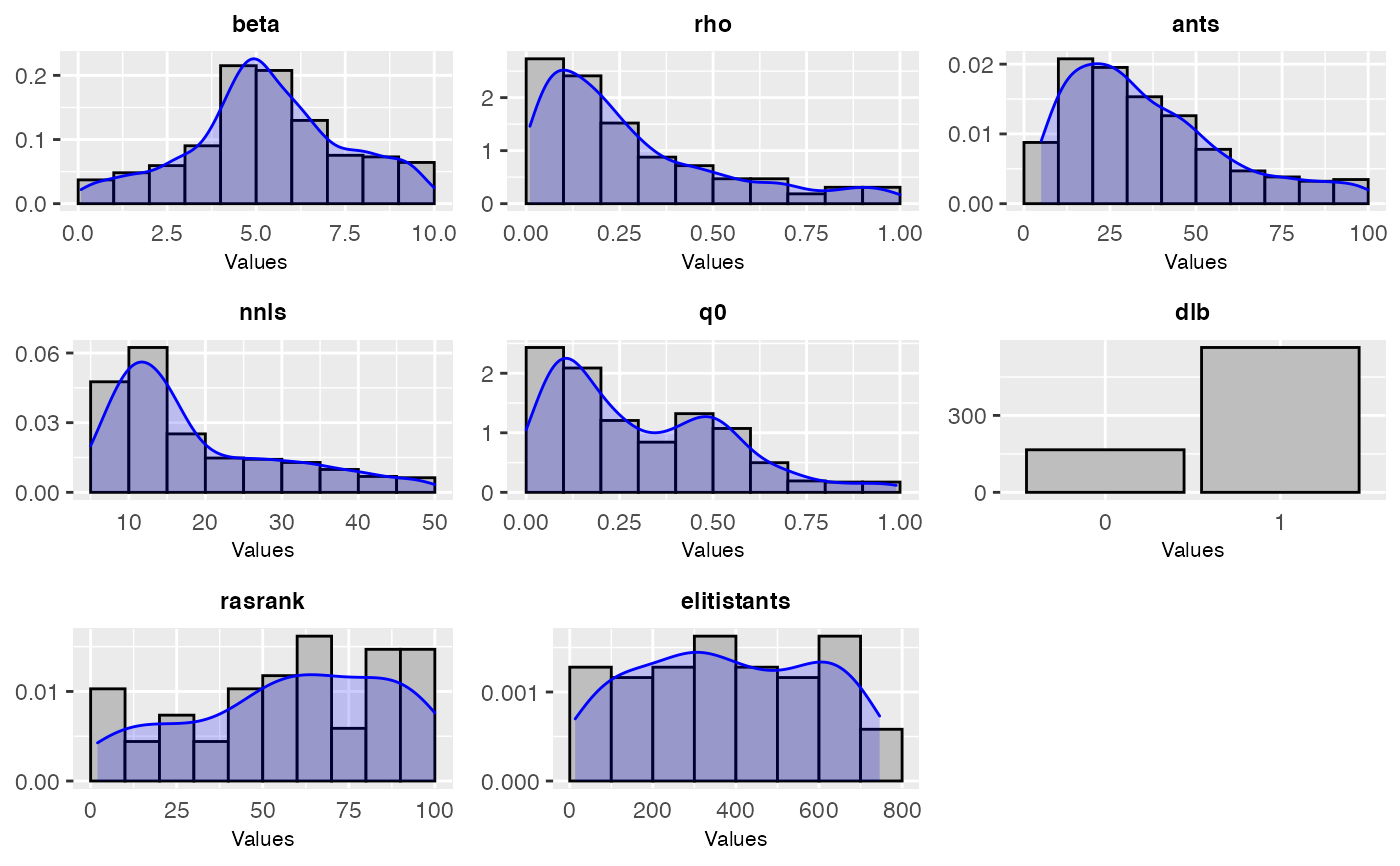
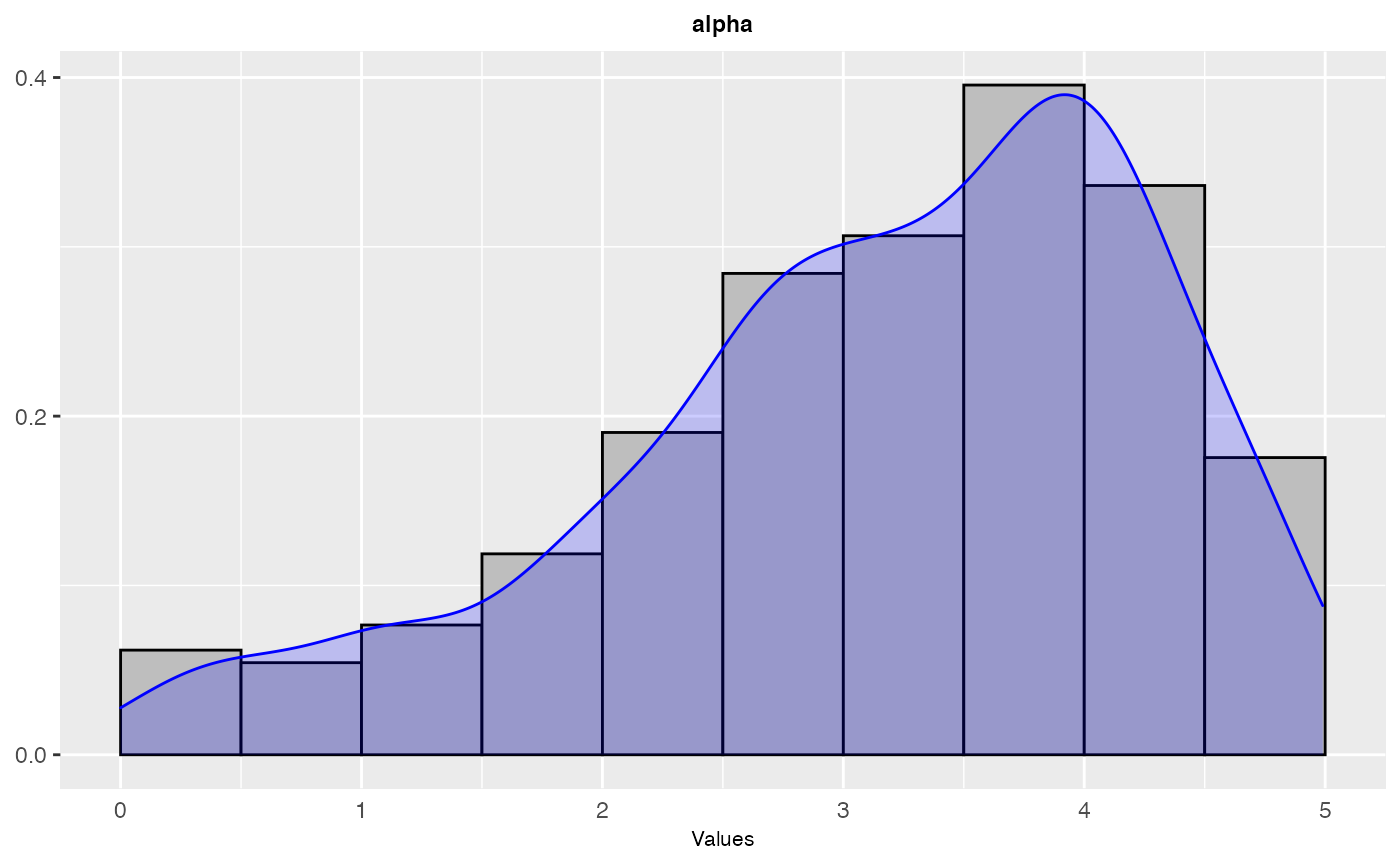
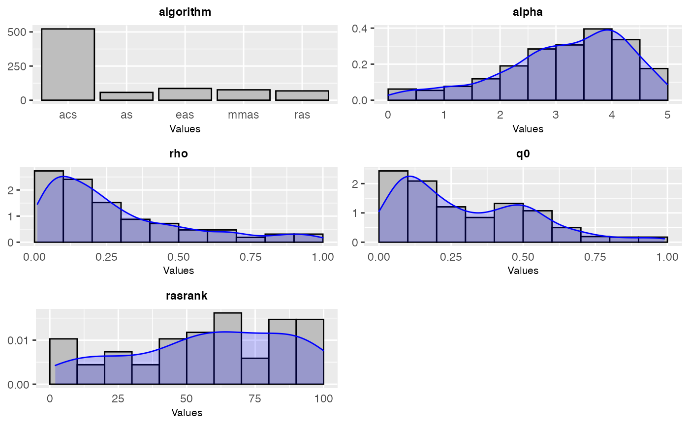
The `sampling_frequency` function creates a frequency or density plot that depicts the sampling performed by irace across the iterations of the configuration process.
For categorical parameters a frequency plot is created, while for numerical parameters a histogram and density plots are created. The plots are shown in groups of maximum 9, the parameters included in the plot can be specified by setting the param_names argument.
sampling_frequency(
  irace_results,
  param_names = NULL,
  n = NULL,
  file_name = NULL
)
Arguments
| irace_results | The data generated when loading the |
|---|---|
| param_names | String vector, A set of parameters to be included (example: param_names = c("algorithm","alpha","rho","q0","rasrank")) |
| n | Numeric, for scenarios with large parameter sets, it selects a subset of 9 parameters. For example, n=1 selects the first 9 (1 to 9) parameters, n=2 selects the next 9 (10 to 18) parameters and so on. |
| file_name | String, file name to save plot. If there are more than 9 parameters, a pdf file extension is recommended as it allows to create a multi-page document. Otherwise, you can use the n argument of the function to generate the plot of a subset of the parameters. (example: "~/path/to/file_name.pdf") |
Value
Frequency and/or density plot
Examples
sampling_frequency(iraceResults)sampling_frequency(iraceResults, n = 2)#> TableGrob (3 x 3) "arrange": 8 grobs #> z cells name grob #> 1 1 (1-1,1-1) arrange gtable[layout] #> 2 2 (1-1,2-2) arrange gtable[layout] #> 3 3 (1-1,3-3) arrange gtable[layout] #> 4 4 (2-2,1-1) arrange gtable[layout] #> 5 5 (2-2,2-2) arrange gtable[layout] #> 6 6 (2-2,3-3) arrange gtable[layout] #> 7 7 (3-3,1-1) arrange gtable[layout] #> 8 8 (3-3,2-2) arrange gtable[layout]#> TableGrob (3 x 2) "arrange": 5 grobs #> z cells name grob #> 1 1 (1-1,1-1) arrange gtable[layout] #> 2 2 (1-1,2-2) arrange gtable[layout] #> 3 3 (2-2,1-1) arrange gtable[layout] #> 4 4 (2-2,2-2) arrange gtable[layout] #> 5 5 (3-3,1-1) arrange gtable[layout]