Introduction
The iraceplot package provides a set of functions to create plots to visualize the configuration data generated by the configuration process implemented in the irace package.
The configuration process performed by irace will show ar the end of the execution one or more configurations that are the best performing configurations found. This package provides a set of functions that allow to further assess the performance of these configurations and provides support to obtain insights about the details of the configuration process.
Installation
Install iraceplot
For installing iraceplot you need to install the devtools package:
install.packages("devtools")Currently, the iraceplot package can be installed from Github:
devtools::install_github("pabloOnate/iraceplot")How to use
This is a basic example that shows how to use iraceplot:
To use the functions its required to have the log file generated by irace (logFile option in the irace package), commonly saved in the in the directory in which irace was executed with the name irace.Rdata. To load the irace log data, replace the path of the file with yours:
load("~/path/to/irace.Rdta")This file contains the iraceResults variable which contains the irace log. For more details about this variable, please go to the documentation of the irace package.
Executing irace
To use the methods provided by this package you must have an irace data object, this object is saved as an Rdata file (irace.Rdata by default) after each irace execution.
During the configuration procedure irace evaluates several candidate configurations (parameter settings) on different training insrances, creating an algorithm performance data set we call the training data set. This information is thus, the data that irace had access to when configuring the algorithm.
You can also enable the test evaluation option in irace, in which a set of elite configurations will be evaluated on a set of test instances after the execution of irace is finished. Nota that this option is not enabled by default and you must provide the test instances in order to enable it. The performance obtained in this evalaution is called the test data set. This evaluation helps assess the results of the configuration in a more “real” setup. For example, we can assess if the configuration process incurred in overtuning or if a type of instance was underrepresented in the training set. We note that irace allows to perform the test evaluations to the final elite configurations and to the elite configurations of each iterations. For information about the irace setup we refer you to the irace package user guide.
Note: Before executing irace, consider setting the test evaluation option of irace.
Once irace is executed, you can load the irace log in the R console as previously shown.
Visualizing irace configuration data
In the following, we provide an example how these functions can be used to visualize the information generated by irace.
Configurations
Once irace is executed, the first thing you might want to do is to visualize how the best configurations look like. You can do this with the parallel_coord method.
parallel_coord(iraceResults)This plot shows the final elite configurations settings, each line represents one configuration. Note that the number of iterations is shown in the scale on the right and the final elite configurations belong to the last iteration. To visualize configurations considered as elites in each iteration use the iterations option:
parallel_coord(iraceResults, iterations=1:iraceResults$state$nbIterations)You can also visualize all configurations sampled in one or more iterations disabling the only_elite option. For example, to visualize configurations sampled in iterations 1 to 9:
parallel_coord(iraceResults, iterations=1:9, only_elite=FALSE)The parallel_coord2 function generates a similar parallel coordinates plot when provided with an arbitrary set of configurations without the irace execution context. For example, to display all elite configurations:
all_elite <- iraceResults$allConfigurations[unlist(iraceResults$allElites),]
parallel_coord2(all_elite, iraceResults$parameters)
A similar display can be obtained using the parallel_cat function. For example, to visualize configurations sampled on iterations 3, 4 and 5.
parallel_cat(irace_results = iraceResults, iterations = c(3,4,5) )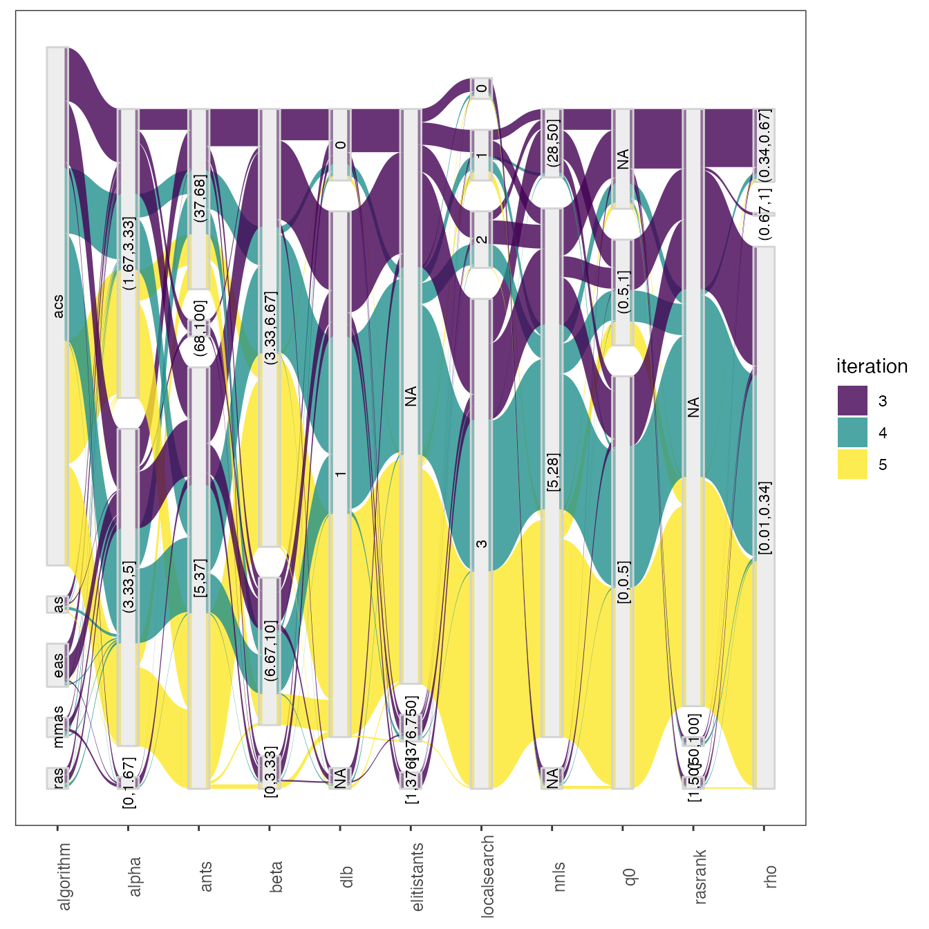
In the parallel_coord and parallel_cat functions parameters can be selected using the param_names arguments. For example to select :
parallel_cat(irace_results = iraceResults,
param_names=c("algorithm", "localsearch", "dlb", "nnls"))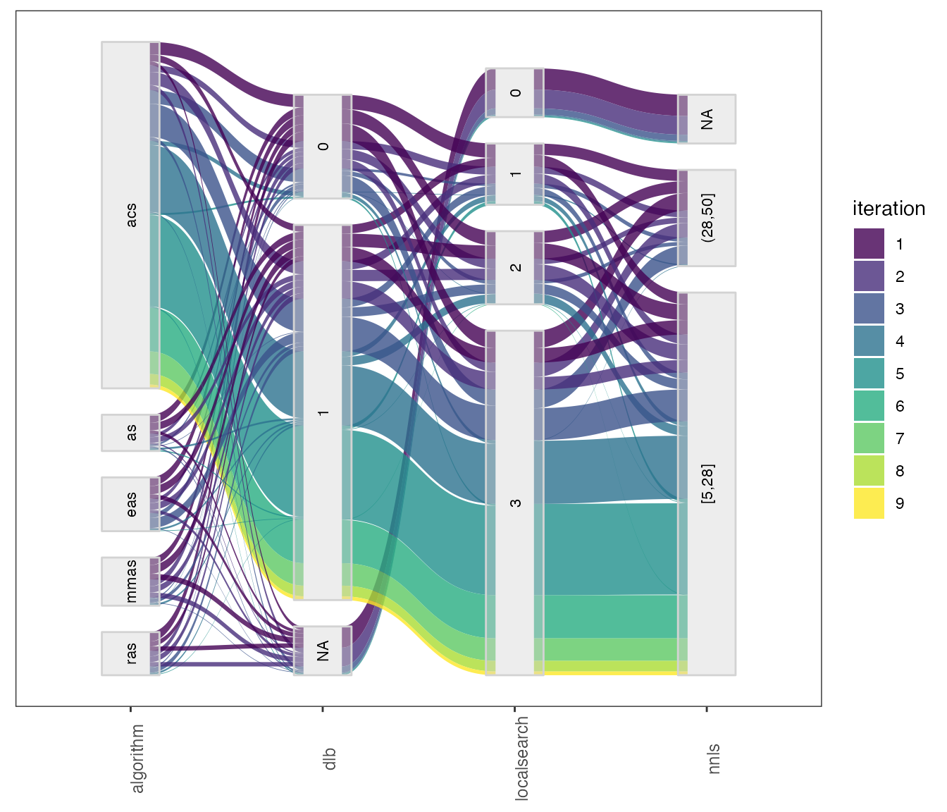 For configuration scenarios that define a large number of parameters, it is impossible to visualize all parameters in one of these plots. The parameters can be split in different plots using the
 by_n_param argument which specifies the maximum number of parameters to include in a plot. The functions will generate as many plots as needed to cover all parameters included.
The sampling_pie function creates a plot that displays the values of all configurations sampling during the configuration process. As well as in the previous plot, numerical parameters domains are discretized to be showm in the plot. The size of each parameter value in the plot is dependent of the number of configurations having that value in the configurations.
sampling_pie(irace_results = iraceResults)Sampled parameter values
In some cases in might be interesting to have a look at the values sampled during the configuration procedure as they show the areas in the parameter space where irace detected a high performance.
A general overview of the samples parameters values can be obtained with the sampling_frequency function which generates frequency and density plots for the sampled values:
sampling_frequency(iraceResults)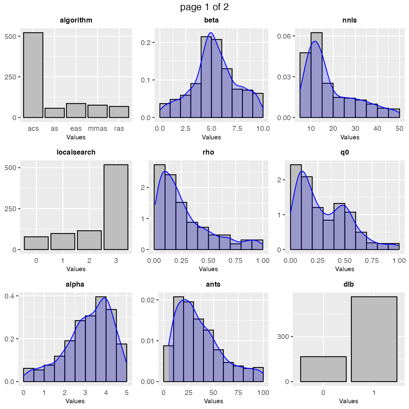
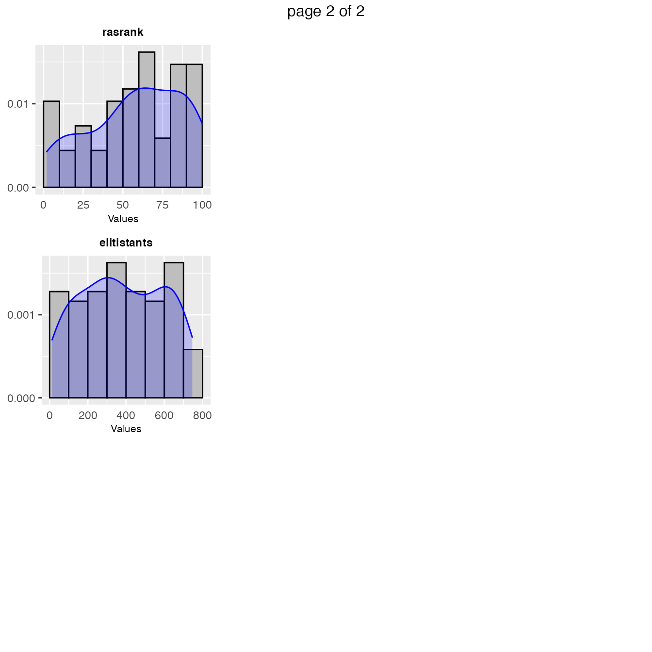 Included parameters specified with the param_names argument. These plots give a general idea of the area of the parameter space in which the sampling performance by irace was focused. For example:
sampling_frequency(iraceResults, param_names = c("beta"))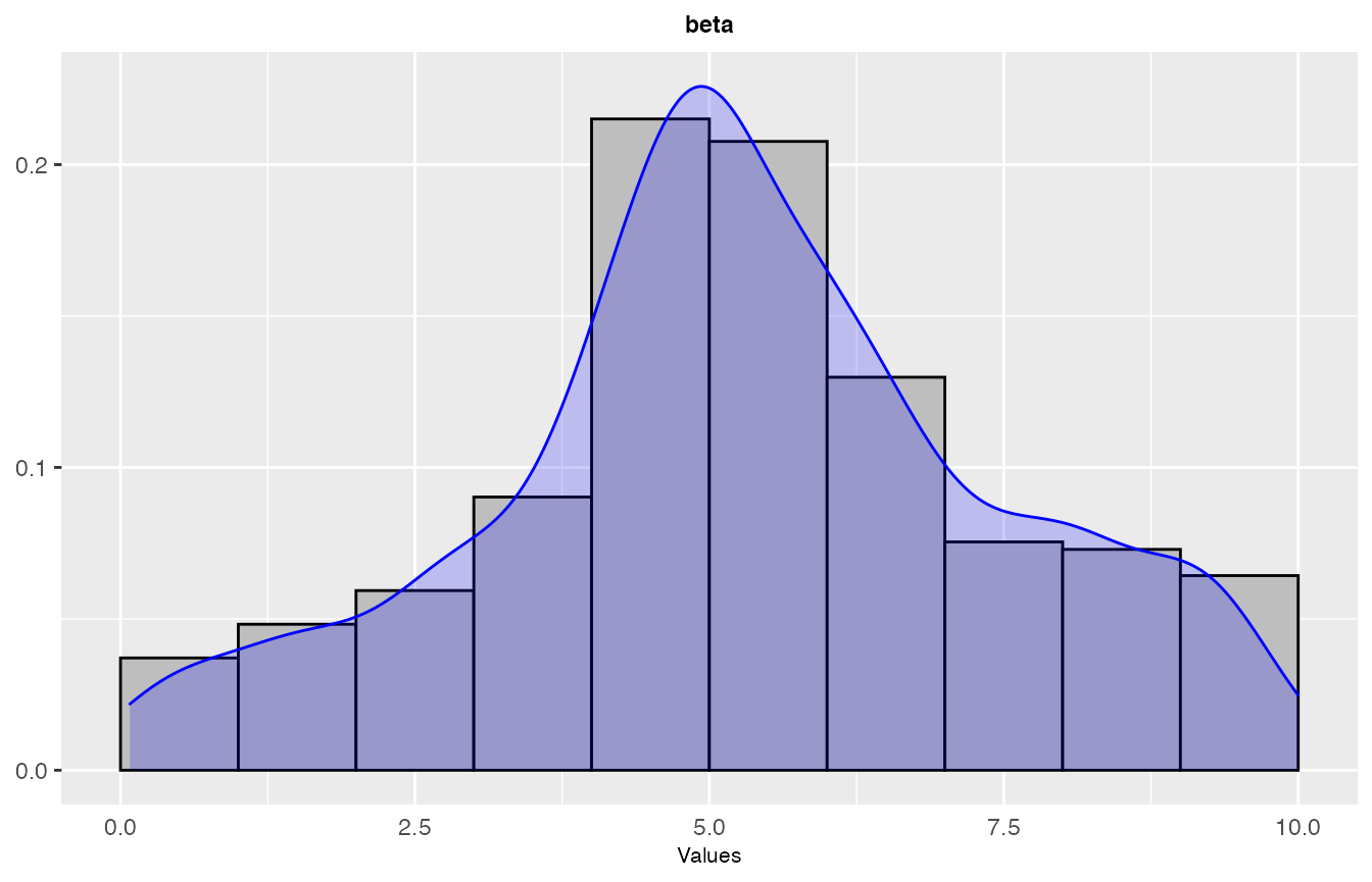
A detailed plot showing the sampling by iteration can be obtained with the sampling_frequency_iteration function. This plot shows the convergence of the configuration process reflected in the sampled parameter values.
sampling_frequency_iteration(iraceResults, param_name = "beta")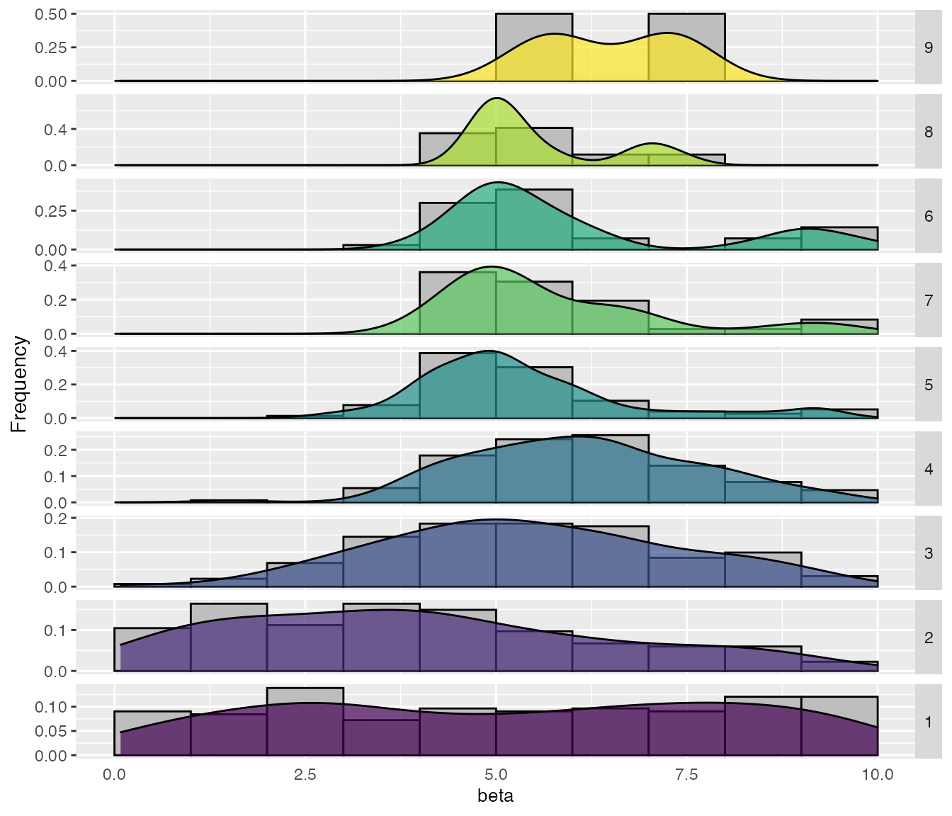
The mean distance between the sampled configurations can be visualized using the sampling_distance function. The argument t defines a percentage used to define a domain interval to assess equality of numerical parameters. For example, if the domain of a parameter is [0,10] and t=0.1 then when comparing any value to v=2 we define an interval s=t* (upper_bound -lower_bound) = 0.1*(10-0)=1. Then all values in the interval [v-s, v+s] [1,3] will be equal to v=2.
sampling_distance(iraceResults, t=0.05)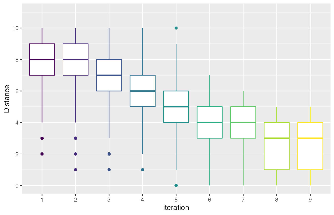
Visualizing Performance
Test performance (elite configurations)
The test performance of the best final configurations can be visualised using the boxplot_test function. Note that the irace execution include test data (test is not enabled by default).
boxplot_test(iraceResults, type="best")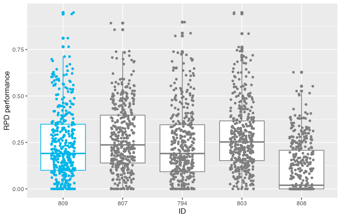
This plot shows all final elite configurations evaluation on the test instance set, we can compare the performance of these configurations to select one that has the best test performance.
If the irace data includes iteration elites, its possible to plot the test performance of elite configurations across the iterations. The best elite configuration on each instance is displayed in blue:
boxplot_test(iraceResults, type="all")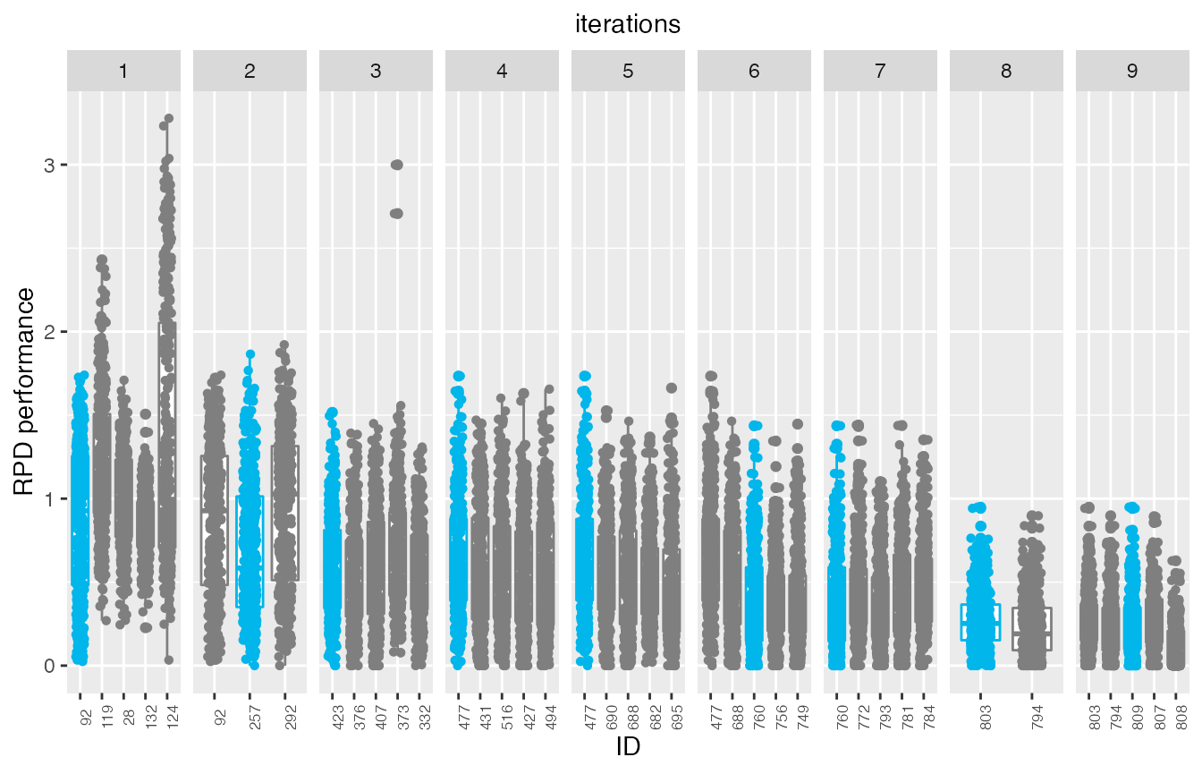
This plot allows to assess the progress of the configuration process regarding the test set performance, which would be useful when dealing with heterogeneous instance sets. In these cases, good configurations across the full set can be challenging to find and it is possible that the algorithm could be mislead if instances sets are prone to introduce bias due to instance ordering.
Note that in this example the elite configuration with id 808 seems to have a slightly better performance
than the configuration identified as the best (id:809) by irace. It is important to note that all elite configurations are not statistically different and thus, its very possible that such situation is observed when evaluuting test performance, specially when configuring heterogeneous, difficult to balance, instance sets.
To investigate the difference in the performance of two configurations the scatter_test function displays the performance of both configurations paired by instance (each point represents an instance):
scatter_test(iraceResults, id_configurations = c(808,809), .interactive=TRUE)This plot can help to identify subsets of instances in which a configuration clearly outperforms other. To further understand the difference of these two configurations the trainig data might be explored to verify if such effect holds for the training set.
Training performance (all configurations)
The following functions create plots of the training data in the irace log. This data is created when executing irace and it is generated by irace when searching for good configurations. Due to the racing procedure, some configurations are more evaluated than others (in general, best configurations are more evaluated). See the irace package documentation for details.
Visualizing training performance might help to obtain insights about the reasoning that followed irace when searching the parameter space, and thus it can be used to understand why irace considers certain configurations as high or low performing.
To visualize the performance of the final elites observed by irace, the boxplot_training function plots the experiments performed on these configurations. Note that this data corresponds to the performance generated during the configuration process thus, the number of instances on which the configurations were evaluated might vary between elite configurations.
boxplot_training(iraceResults)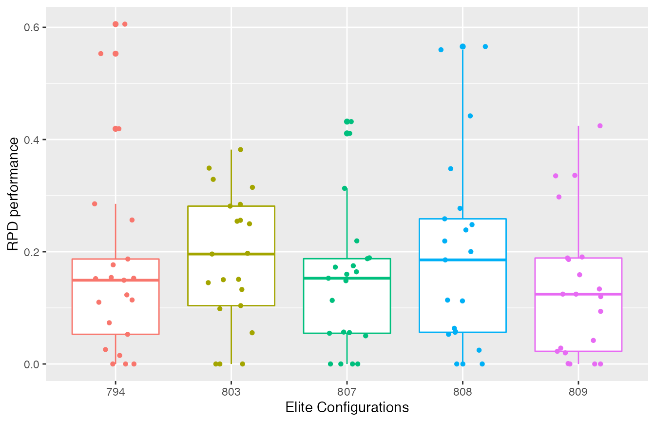
To observe the difference in the performance of two configurations you can also generate a scatter plot using the scatter_training function:
scatter_training(iraceResults, id_configurations = c(808,809), .interactive=TRUE)Visualizing the configuration process
In some cases, it might be interesting have a general visualization for the configuration process. This can be obtained with the plot_experiments_matrix function:
plot_experiments_matrix(iraceResults, .interactive = TRUE)The sampling distributions used by irace during the configuration process can be displayed using the plot_model function. For categorical parameters, this function displays the sampling probabilities associated to each parameter value by iteration (x axis top) in each elite configuration model (bars):
plot_model(iraceResults, param_name="algorithm")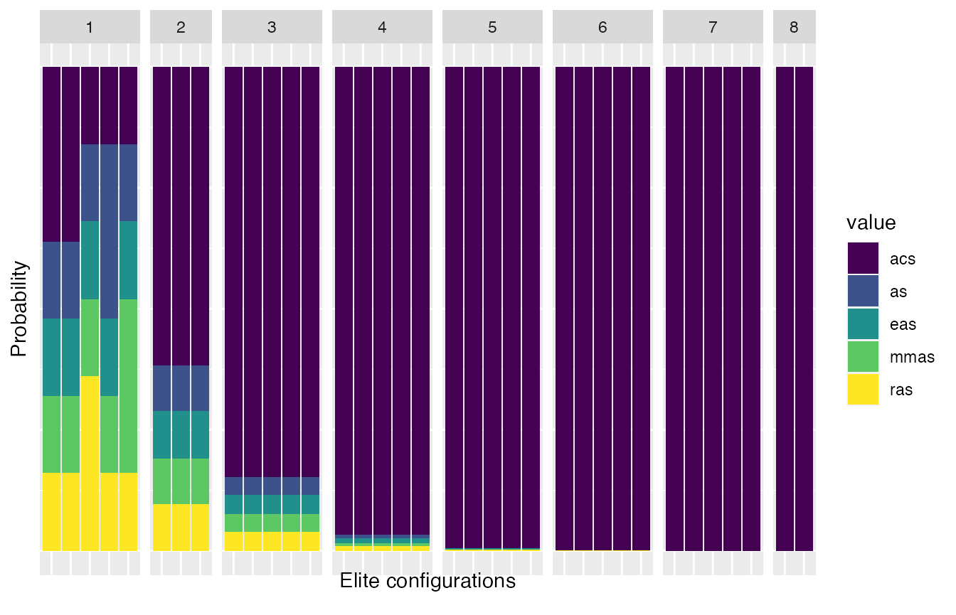
For numerical parameters, this function shows the sampling distributions associated to each parameter. These plots display the the density function of the truncated normal distribution associated to the models of each elite configuration in each instance:
plot_model(iraceResults, param_name="alpha")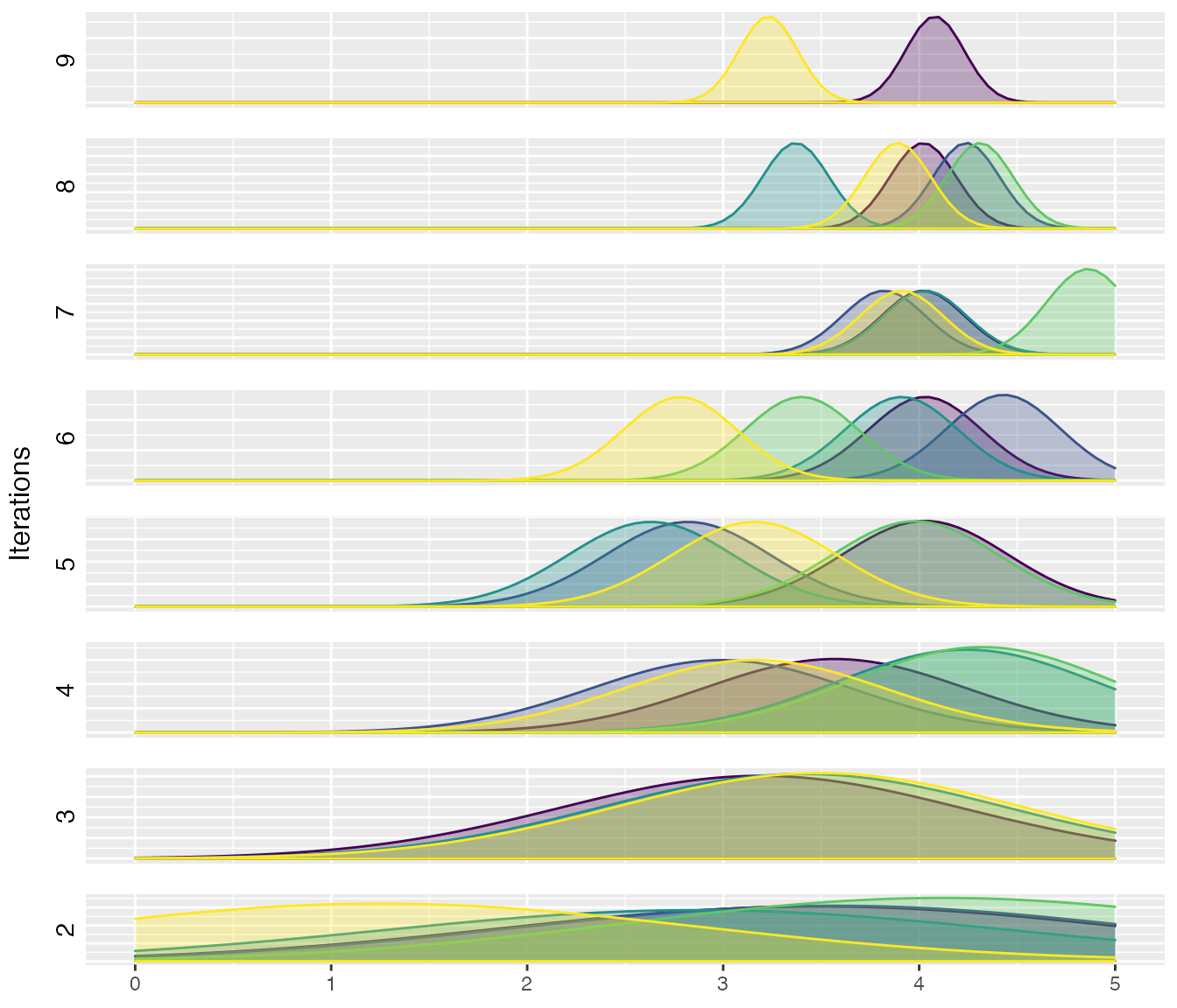
Report
The report function generates an HTML report with a summary of the configuration process executed by irace. The function will create an html file in the path provided in the file_name argument and appending the “.html” extension to it.
report(iraceResults, file_name="report")